Ch 5: Introduction to Programming

Return to all notes

The following are number of advanced techniques in Maple. Again, these are general ideas that appear in any CAS, but the format will be specific to Maple. These allow a user of Maple to create more complicated series of mathematical steps in a nice way. The following techniques are described here:

procedures These are similar to functions that we saw earlier, but allow more complicated steps to occur.
boolean values A boolean is something that is either true or false.
if and while statements An if statement allows a few statements of code to branch depending on some condition. A while statement allows for a few statements of code to continue to run until a condition occurs.
loops A loop is a few statements of code that is run generally a fixed number of times.
recursion Recursion is a type of procedure that allows code to call itself. Although often you can generate code that duplicates recursive code, it is often clearer to understand and often come directly from mathematical statements.

Procedures

A procedure is very similar to a function in any computer language. In Maple, these are similar in that there is a input (or a number of inputs) and the result is some output (numbers, a plot, an expression). In fact, all commands in Maple are just procedures.

Recall that if we have a simple function that returns the square of a number, we can write that as

f(x):=x^2

We can also define a procedure in a similar manner.

F:=proc(x::numeric)::numeric;
  return x^2:
end proc:

A few things to note with this

This is much more complex to write out than the equivalent function.
To get a line inside a procedure without evaluating it, type SHIFT-ENTER
A procedure allow more complicated structures as we will see.
You can call this in the same way, $F(2),F(-2)$ for example.
The types of input is defined for us (these are options). We can only use this to square numbers (integers, decimals, etc.)
You will notice an error if you do $F(x+1)$.

We can use this procedure to square numbers, but not expressions.

Let’s also examine a similar procedure that adds numbers:

add:=proc(x::numeric,y::numeric)::numeric;
   return x+y:
end proc:

Exercises

remove the semicolon and colon off the end of the lines of the procedure, reenter it and see what happens. Can you understand what is going on?
Write a procedure called mult that multiplies two numbers and returns the product.
Write a procedure called average that returns the average of three numbers.

semicolons and colons

Recall that when we loaded a library, we put a colon (:) at the end of the line. This was to suppress the output. That is true about any command in Maple. It also separately two statements as we will see below.

A semicolon can end a command without suppressing output. It is often used to separate statements as well. You will see either colons or semicolons inside of procedures because they are needed. If you get output when you don’t expect it, use a colon.

Boolean values and if statements

A boolean value is something that is either true or false. These are built-in constants in Maple. Sometimes we will want to know if a statement is true or false, but generally, we will use them in other structures.

if statements

An if statement is often used inside of a procedure to do different things depending on the value of a variable. Consider the piecewise version of the absolute value. Mathematically, we write:
$$ |x| = \begin{cases} x & x \geq 0 \newline
-x & x<0
\end{cases} $$

We can make a Maple procedure for the absolute value the following way:

absol := proc(x::numeric)::numeric;
  if x >= 0 then
     return x:
  else
     return -1*x:
  end if:
end proc:

And to help determine if it is correct, evaluate absol(3) and absol(-7).

Exercise

The modulus of an integer is the remainder in division. For example, 7 mod 3 is 1.

Write a procedure call isOdd that take a positive integer (type posint) and returns true if the number is odd and false if not. Use the modulus with the divisor 2.

Loops

A loop is a series of statements that are repeated either a fixed number of times or until a condition occurs. They can be very helpful if a large number of operations need to be done in a predictable manner.

while loops

Another very common construction for programming is called a while loop. Basically, we want to run a few statements while some boolean statement is true. Here’s a simple example:

n:=1:
while n<10 do
  print(n):
  n:=n+1:
end do:

And that isn’t very interesting, but we can reproduce the seq command crudely in the following way. Let’s say we want to return a list of numbers from 1 to $n$, where $n$ is a positive integer.

intList := proc (n::posint)::list;
   local list := []:
   local i := 1:
   while i <= n do
     list := [op(list), i]:
     i := i+1:
   end do:
   return list:
end proc:

A few things to note about this:

Putting local in front of a variable tells Maple the variables are local to the procedure. That is, don’t use the values outside the procedure if they exist.
The line list:=[op(list), i] simply adds the value of i to the end of the list. Other languages have a push command to do this.
The op command in the line strips the brackets off of the list, returning a sequence.

Let’s run some examples:

typing intList(6) returns [1,2,3,4,5,6]
typing intList(10) returns [1,2,3,4,5,6,7,8,9,10]

The following is a more interesting example. If you have a positive integer $n$, the following returns a list of all factors of $n$. Recall that for a positive integer $n$, the factors of $n$ are all numbers that divide $n$ with 0 remainder. Both 1 and $n$ are always factors of $n$.

allfactors:=proc(num::posint)::posint;
  local factors := [1]:
  local n := 2:
  while n <= num do
    if num mod n = 0 then
      factors := [op(factors), n]:
    end if:
    n := n+1:
  end do:
  return factors:
end proc:

And here’s a couple of examples of this

type allfactors(6) returns [1,2,3,6]
type allfactors(29) returns [1,29]

Another possible procedure that you want is to determine if a number is prime. Although this is built-in, let’s find a way to do this using the allfactors command.

isPrime := proc(n::posint)::boolean;
  local factors := allfactors(n);
  return evalb(factors[2] = n)
end proc:

Alternatively, prime numbers have only 2 numbers in factor list and so it can be checked if the length (using the nops, for number of operands, command) is 2.

isPrime := proc(n::posint)::boolean;
  return evalb(nops(allfactors(n))=2)
end proc:

where evalb will return true or false instead of (perhaps) the equation. Note that this nests a number of commands that could be done as steps.

Another nice use of all factors is the use of a theorem that says that the total number of factors is even (factors pair up) unless the number is a perfect square. We will then use this and the isOdd function you wrote above to write an isPerfectSquare procedure.

isPerfectSquare := proc(n::nonnegint)::truefalse;
  if isOdd(nops(allfactors(n))) then
    return true
  else
    return false
  end if
end proc:

or to even shorten this more, we can write this as:

isPerfectSquare := proc(n::nonnegint)::truefalse;
  return isOdd(nops(allfactors(n)))
end proc:

Infinite Loops

It is common in a while loop to keep running it forever. This occurs if you don’t have some code that will stop it. A couple of things:

Make sure something is changing in your loop. If you intend to stop the loop on an index, make sure the index is updating.
Look at your code and see if you have something that you think will stop the loop. What ever is in the boolean statement needs to eventually switch.
Stop the code if you need to. Maple has a Stop Sign on the toolbar. This will interrupt the kernel. Often you will need to do this, but this may not actually give you control back. You can also restart the kernel using the circle arrow on the toolbar.
If you can’t figure out why it is in an infinite loop, put print statements inside to print out values of variables.

Compound booleans in an `if` statement or `while` loop

Recall that a boolean is something that evaluates to true or false and is needed in an if statement or while loop. Often more than one boolean is needed. This is called a compound boolean and is created with either an and or an or.

An or compound statement. If either or both are true, the result is true, otherwise false.
- true or true is true
- true or false is true
- false or true is true
- false or false is false
An and compound statement. Both must be true to be true, otherwise false
- true and true is true
- true and false is false
- false and true is false
- false and false is false

Here’s an example, where we just print out all odd perfect squares less than 100. (Note: there is a better way to do this, but the point is to show how to use a compound statement)

n:=1:
while n<=100 do
  if isOdd(n) and isPerfectSquare(n) then
    print(n)
  end if:
  n:=n+1:
end do:

In addition, the not command switches a true to false and a false to true. A simple version of this would be if we had an isOdd function as written above, then the following would be an isEven function:

isEven:=proc(n::nonnegint)::truefalse;
  return not isOdd(n)
end proc:

More functions with prime numbers

We want to find the smallest prime number bigger than a number n. We will make a procedure that return the next prime.

theNextPrime := proc(n::integer)::integer;
  local k := n+1:
  while not(isPrime(k)) do
     k := k+1
  end do:
  return k:
end proc:

Exercise

A perfect number is a positive integer $n$, that has the property that the sum of the factors (other than $n$ itself) equals $n$. We will write a few procedures here to find perfect numbers.

Write a procedure called isPerfect which takes a positive integer, $n$ and return either true or false on whether or not $n$ is a perfect number. (Hint: use the built-in function add which will take a list of numbers and return the sum.)
Test your procedure on some known perfect numbers (6 and 28) and others (like all other numbers less than 100 are not perfect.)
Write a procedure called nextPerfect which takes an integer, $n$ and return the next perfect number greater than $n$.
Test your procedure to find the first few perfect numbers. (Don’t go too big or Maple will bog down. )

For loops

The following is a simple for loop that prints out the numbers 1 to 10

for i from 1 to 10 do
  print(i):
end do:

If you want to skip numbers or count backwards, the following

for i from 1 by 2 to 19 do
  print(i):
end do:

for i from 10 by -1 to 1 do
  print(i):
end do:

and the following adds numbers in a list.

s := 0;
for i in [3, 5, 7, 11, 13, 19] do
  s := s+i
end do

Note: there is a command called add that will also do the above.

add([3,5,7,11,13,19])

This isn’t a very interesting example, but shows the syntax of a for loop. Often a for loop is used in conjunction with a procedure. Above, we used a while loop to create an integer list. However, it was a loop with a fixed number of steps in which a for loop is better to use. Here’s a different way to create the integer list:

intList := proc(n::posint)::list;
   local li := [];
   local i;
   for i to n do
     li := [op(li), i]
   end do;
   return li
end proc

Also, there are two variables that live inside the procedure: i and li. Because they are not needed outside the procedure, we declare them local. If you don’t declare them as local, Maple will give a warning.

If Maple didn’t have a factorial builtin, here’s a way we could handle it.

facty:=proc(n::nonnegint)::posint;
   local i,fact:=1:
   for i from 1 to n do
     fact:=fact*i:
   end do:
   return fact:
end proc:

and the heart of this is that the for loop multiplies all of the numbers from 1 to n together (it does this one step at a time).

Note: if you call this function factorial, you will get a warning from Maple, which is why it is called facty.

While Loops Versus For Loops

No this, isn’t a smackdown between these two. A big question often is when should I use a while loop and when should I use a for loop. The general rule of thumb is:

If you know that you need to run code for a fixed number of times, use a for loop
If you need to do something in a list and map doesn’t work well, use a for loop.
If you don’t use a while loop. Generally, the doing something in the loop will affect how many times the loop is run.

Types

All of these procedures have the arguments and return typed. That is, it is important to say what type of Maple object you can pass it. Here’s a list of many common types:

integer: the standard mathematical integer
posint: positive integer. That is 1,2,3,…
negint: negative integer. That is, -1, -2, -3, ….
nonnegint: non negative integer, 0, 1, 2, 3 …
nonposint: non-positive integer: 0,-1,-2,-3,…
rational: rational (fraction) number.
realcons: a real constant
numeric: a number (integer, real, rational)
truefalse: a boolean (a true or false value)
list: a list, like [1,2,3]
procedure: a mathematical function.
range: an interval, like 1..2 all numbers between 1 and 2.

Recursion

Above, we saw how to compute the factorial of a number using a for loop. There’s another way to do this. We can define the factorial in the following way:
$$ n!=\begin{cases}1&n=0\newline n\cdot(n-1)!&\text{otherwise}\end{cases}$$

The big difference is that inside the function is a call to the function. This is what is called a recursive function. Often this is very helpful and the factorial is a great example of this. We can write the factorial this way in the following:

factr := proc(n::nonnegint)::posint;
   if n = 0 then
      return 1
   else
      return n*factr(n-1);
   end if
end proc:

or using the ifelse function:

factr := proc(n::nonnegint)::posint;
   return ifelse(n=0,1,n*factr(n-1));
end proc:

Exercise

Try the function factr for various values of $n$.
Compare the results to the built-in factorial !.

Another Fun Recursive example

Here’s another fun example. A number $n$ is called happy by the following
1. Take the digits of $n$ and square each one.
2. Sum the squares.
3. if the sum is 1, then the number is happy, if not repeat these steps.

Note: it’s also helpful that if this process results in the number 4, then you can never result in a sequence that reaches 1. You can call these number unhappy.

The number 13 is a happy number because $1^{2}+3^{2}=10$ and $1^{2}+0^{2}=1$, so the result ends in 1.
The number 19 is also happy because $1^{2}+9^{2}=1+81=82$, then $8^{2}+2^{2}=64+4=68$, then $6^{2}+8^{2}=36+64=100$, then $1^{2}+0^{2}+0^{2}=1$.
The number $4$ isn’t happy because $4^{2}=16$, then $1^{2}+6^{2}=1+36=37$, then $3^{2}+7^{2}=9+49=58$, then $5^{2}+8^{2}=25+64=89$, then $8^{2}+9^{2}=64+81=145$, then $1^{2}+4^{2}+5^{2}=1+16+25=42$, then $4^{2}+2^{2}=16+4=20$, then $2^{2}+0^{2}=4$ and since we have returned to 4, this will continue cycling, so we stop and say 4 is unhappy.
It has been proven that any unhappy number will eventually hit this cycle.

To write this in Maple, first, it is helpful to have a procedure that splits any positive integer into its digits. Hereܙs such a procedure:

splitDigits := proc(n::posint)::list;
   local list := [], k := n;
   while 9 < k do
      list := [k mod 10, op(list)];
      k := iquo(k, 10)
   end do;
   return [k, op(list)]
end proc:

and test this a bit using some 3 and 4 digits numbers.

Then we can write a isHappy procedure in the following way.

isHappy := proc(n::posint)::truefalse;
  local squares, sum:
  if n = 1 then return true end if;
  if n = 4 then return false end if;
  squares := map(k->k^2,splitDigits(n)):
  sum := add(squares):
  return isHappy(sum):
end proc:

A few things about this:

note that this is recursive in that it calls itself.
The last three list can be written compactly as

return isHappy(add(k^2, k in splitDigits(n)))

Let’s now say that we wish to find all numbers less than 100 that are happy. To run this command on every number between 1 and 100, can be done many ways. A for loop comes to mind, but using the seq command is better:

allhappies:=[seq(isHappy(n),n=1..100)]

and you will see a list of true or false and perhaps that isn’t that helpful. We can use the Search and SearchAll commands in the ListTools package to help us out.

with(ListTools)

and if we have the list

letters:=["a","c","a","e","f","f","a"]

We can use Search to find where the letter “a” is

Search("a", letters);

and this returns 1. If instead we use

SearchAll("a", letters);

we get 1,3,7, which are the locations of the “a"s above.

So if we use

SearchAll(true,allhappies)

we get a list of all of the happy numbers up to 100.

Exercise

A fibonacci number is defined as $F(1)=1, F(2)=1$, then $F(n)=F(n-1)+F(n-2)$ for $n \geq 3$. This is naturally a recursive function. Write a procedure $F$ that take a positive integer $n$ and returns the $n$th Fibonacci number using recursion. Find the first 20 Fibonacci number (hint: use the seq command)

Rootfinding techniques

Before continuing with this chapter, we look at a way to find the zeros (or roots) of a function. Although Maple (and most CASs) have this built-in, we examine the details here.

Consider the function $f(x)=x^{2}-2$, which is plotted below:

$Plot of $x^{2}-2$$

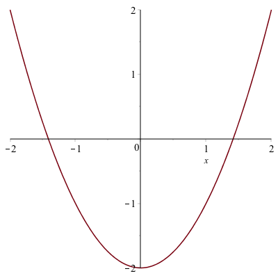
It has two roots $x=\sqrt{2}$ and $x=-\sqrt{2}$. We will use this example to find a numerical approximation of this.

If we evaluate the function at $x=0$ and $x=2$, note that $f(0)=-2$ and $f(2)=2$. The intermediate value theorem states that if a function $f$ is continuous on an interval $[a,b]$, then $f$ takes on all values ($y$-values or heights) between $f(a)$ and $f(b)$. Specifically if $d$ is between $f(a)$ and $f(b)$, then there exists at least one value $c$ such that $f( c )=d$. See this page for more information.

For this example, $f$ is continuous, so $f$ takes on all values between $f(0)=-2$ and $f(2)=2$, including 0. That is, there is a number $c$ such that $f( c )=0$. The value of $c$ is the root we seek.

Bisection Method

The bisection method exploits the intermediate value theorem to make sure that we always have a interval that contains a root. First, we will walk through the bisection method for the example and then write it down in general.

Let $\tilde{a}$ be the midpoint between $a$ and $b$ or $x=0$ and $x=2$ in our case. That is
$$\tilde{a} = \frac{a+b}{2} = \frac{0+2}{2}=1$$
There are three choices for $\tilde{a}$. Either it is 0, then you have found the root or it is less than zero or greater than zero. Since $f(1)=-1$, then it is less than zero. Because our left endpoint was less than zero, we replace it with zero. That is our interval goes from $[0,2]$ to $[1,2]$.

And then we repeat. The midpoint of this interval is 1.5 and $f(1.5)=1.5^{2}-2=0.25$ and since this is positive, we replace the 2 with 1.5 and our new interval is $[1,1.5]$.

Exercise

Find the next 3 intervals using this technique. Recall that you always need to have the function value of one side be less than and the other be greater than 0.

Stop this crazy thing!!!

Since you are wise, you notice that you can continue this process forever and you just don't have that much time. For example, on the tenth iteration, you should have the interval

[1.41406250,1.416015625]

and as long as the condition that the function values of two endpoints are opposite signs, then there is a guarantee of a root inside this interval.

Again, we can go on forever, but a good place to stop (often called a halting condition) is when the length of the interval shrinks to a particular size. Let’s say that we stop when the length is $10^{-4}$ and then we should return our best guess at the root, which may be the midpoint of the final interval. If we stop when the interval is less than $10^{-4}$ and take this midpoint, the answer will be 1.414215088.

Creating a Procedure to do this

This section will slowly build up a procedure that does this. The goal of this section is to learn how to take an algorithm (explained above) and make a procedure that does this.

Shell of a procedure. Let’s start with the declaration of the procedure. We want to take a function and an interval in and return an approximate root.

bisect:=proc(f::procedure,interval::range)::numeric;

end proc:

This will just do that.  Note that a function type is called a `procedure` and an interval is called a `range`.  The return type will be a number, so `numeric`.  It&#8217;s a good idea to just run this at this point.

Define the midpoint and return it.

Next, let’s do something super simple and define the midpoint and then return it. To get the endpoints of an interval or range, use lhs and rhs, which stands for left hand side and right hand side respectively.

bisect:=proc(f::procedure,interval::range)::numeric;
   local mid:=0.5*(lhs(interval)+rhs(interval)):
    return mid:
end proc:

and then execute this block of code.  Make sure there are no errors.  Then you can test it using the example above by typing

bisect(x->x^2,0..2)

and you should get the answer 1.0.

Create a new interval

Now, let’s also create a variable called inter that is the new interval. Recall that you want to make sure that the endpoints of the new interval are opposite signs. The easiest way to check this is to determine if the product of the function values is negative.

bisect:=proc(f::procedure,interval::range)::numeric;
   local mid:=0.5*(lhs(interval)+rhs(interval)):
   local inter:=interval:
   if f(lhs(inter))*f(mid) < 0 then
       inter := lhs(inter) .. mid
   else
      inter := mid .. rhs(inter)
   end if:
   return inter:
end proc:

If we test this with `bisect(x->x^2-2,0..2)` we get

1.0 .. 2

which means that the root is in the interval [1.0,2.0].

Put in a loop to run a few times.

Next, we will run this a few times using a for loop to test the procedure.

bisect:=proc(f::procedure,interval::range)::numeric;
   local mid:=0.5*(lhs(interval)+rhs(interval)):
   local inter:=interval:
   local i:

   for i to 4 do
     if f(lhs(inter))*f(mid) < 0 then
       inter := lhs(inter) .. mid
     else
       inter := mid .. rhs(inter)
     end if:
     mid := .5*(lhs(inter)+rhs(inter)):
     print(inter):
    end do;
  return mid
end proc:

This will print out the interval to make sure it is working.  You should see the interval printed 4 times and then the midpoint returned (and then printed):

1.0 .. 2
1.0 .. 1.50
1.250 .. 1.50
1.3750 .. 1.50
1.43750

so this appears that the root is 1.43750 and is guaranteed to be in the interval [1.375,1.5]

Replace the for loop with a while loop

We don’t want to run this a fixed number of times, but instead, run this until the halting condition.

We will execute the loop while the length of the interval is greater than $10^{-4}$.

bisect := proc (f::procedure, interval::range)::numeric;
  local mid := .5*(lhs(interval)+rhs(interval));
  local inter := interval;
  while rhs(inter)-lhs(inter) > 10^(-4) do
    if f(lhs(inter))*f(mid) < 0 then
      inter := lhs(inter) .. mid
    else
      inter := mid .. rhs(inter)
    end if;
    mid := .5*(lhs(inter)+rhs(inter));
    print(inter):
  end do;
  return mid:
end proc:

If we test the procedure by typing: `bisect(x->x^2-2,0..2)`, you will get 1.414215088.  Note that we can determine the number of digits of accuracy for $\sqrt{2}$ by typing

evalf(|sqrt(2)-1.414215088|)

will result in 0.000001526 or 5 digits of accuracy.

Adding a parameter for the halting condition.

If we want the halting condition to be smaller than $10^{-4}$, we will make it a parameter. Here’s how that works.

bisect := proc (f::procedure, interval::range,{eps:=10^(-4)})::numeric;
  local mid := .5*(lhs(interval)+rhs(interval));
  local inter := interval;
  while rhs(inter)-lhs(inter) > eps do
    if f(lhs(inter))*f(mid) < 0 then
      inter := lhs(inter) .. mid
    else
      inter := mid .. rhs(inter)
    end if;
    mid := .5*(lhs(inter)+rhs(inter));
  end do;
  return mid:
end proc:

and we have removed the print statement because all seems to be working well.  Now if we call this procedure as above,

bisect(x->x^2-2,0..2)

then we get the same result as above.

But this allows us to get more precision.  Type

bisect(x->x^2-2,0..2,eps=10^(-7))

gives this time 8 digits of accuracy.

Adding some help and error checking to this

It’s often helpful to add a description to the function, so here’s the final result:

bisect := proc (f::procedure, interval::range,{eps:=10^(-4)})::numeric;
  description "This procedure performs the bisection method on the function f with given range.  The parameter eps will determine  the halting condition."
  local mid := .5*(lhs(interval)+rhs(interval));
  local inter := interval;
  if f(rhs(inter))*f(lhs(inter))>0 then
     error "A root is not guaranteed to be in this interval.":
  end if:
  while rhs(inter)-lhs(inter) > eps do
    if f(lhs(inter))*f(mid) < 0 then
      inter := lhs(inter) .. mid
    else
      inter := mid .. rhs(inter)
    end if;
    mid := .5*(lhs(inter)+rhs(inter));
  end do;
  return mid:
end proc:

The description is helpful to remember what the function does.  If you type:

Describe(bisect)

You will see

# This procedure performs the bisection method on the function f with given
# range.
# The parameter eps will determine the halting condition.
# The procedure returns the root of the function f within the given interval
# such that the
# interval is no wider than eps.
bisect( f::procedure, interval::range,
    { eps := .1e-3 } ) :: numeric

and give a brief description of the function.

Also, we now have error checking built it.

We will use this procedure in a homework problem.

Ch 5: Introduction to Programming

Procedures

Exercises

semicolons and colons

Boolean values and if statements

if statements

Exercise

Loops

while loops

Infinite Loops

Compound booleans in an if statement or while loop

More functions with prime numbers

Exercise

For loops

While Loops Versus For Loops

Types

Recursion

Exercise

Another Fun Recursive example

Exercise

Rootfinding techniques

Bisection Method

Exercise

Stop this crazy thing!!!

Creating a Procedure to do this

Compound booleans in an `if` statement or `while` loop